Following from the first part of the tutorial on implementing RNNs , this second part will show how to train a more complex RNN with input data stored as a tensor and trained with RMSProp and Nesterov momentum .
This is the last part of a 2-part tutorial on how to implement an RNN from scratch in Python and NumPy:
# Imports
%matplotlib inline
%config InlineBackend.figure_formats = ['svg']

import itertools
import numpy as np  # Matrix and vector computation package
import matplotlib
import matplotlib.pyplot as plt  # Plotting library
import seaborn as sns  # Fancier plots

# Set seaborn plotting style
sns.set_style('darkgrid')
# Set the seed for reproducability
np.random.seed(seed=1)
#
Binary addition dataset stored in tensor
This tutorial uses a dataset of 2000 training samples to train the RNN that can be created with the
create_dataset
method defined below. Each sample consists of two 6-bit input numbers $(x_{i1}$, $x_{i2})$ padded with a 0 to make it 7 characters long, and a 7-bit target number ($t_{i}$) so that $t_{i} = x_{i1} + x_{i2}$ ($i$ is the sample index). The numbers are represented as
binary numbers
with the
most significant bit
on the right (least significant bit first). This is so that our RNN can perform the addition form left to right.
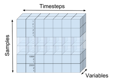
The input and target vectors are stored in a 3th-order tensor. A
tensor
is a generalisation of vectors and matrices, a vector is a 1st-order tensor, a matrix is a 2nd-order tensor. The order of a tensor is the dimensionality of the array data structure needed to represent it.
The dimensions of our training data (
X_train
,
T_train
) are printed after the creation of the dataset below. The first order of our data tensors goes over all the samples (2000 samples), the second order goes over the variables per unit of time (7 timesteps), and the third order goes over the variables for each timestep and sample (e.g. input variables $x_{ik1}$, $x_{ik2}$ with $i$ the sample index and $k$ the timestep). The input tensor
X_train
is visualised in the following figure:
The following code block initialises the dataset.
# Create dataset
nb_train = 2000  # Number of training samples
# Addition of 2 n-bit numbers can result in a n+1 bit number
sequence_len = 7  # Length of the binary sequence

def create_dataset(nb_samples, sequence_len):
    """Create a dataset for binary addition and
    return as input, targets."""
    max_int = 2**(sequence_len-1) # Maximum integer that can be added
     # Transform integer in binary format
    format_str = '{:0' + str(sequence_len) + 'b}'
    nb_inputs = 2  # Add 2 binary numbers
    nb_outputs = 1  # Result is 1 binary number
    # Input samples
    X = np.zeros((nb_samples, sequence_len, nb_inputs))
    # Target samples
    T = np.zeros((nb_samples, sequence_len, nb_outputs))
    # Fill up the input and target matrix
    for i in range(nb_samples):
        # Generate random numbers to add
        nb1 = np.random.randint(0, max_int)
        nb2 = np.random.randint(0, max_int)
        # Fill current input and target row.
        # Note that binary numbers are added from right to left,
        #  but our RNN reads from left to right, so reverse the sequence.
        X[i,:,0] = list(
            reversed([int(b) for b in format_str.format(nb1)]))
        X[i,:,1] = list(
            reversed([int(b) for b in format_str.format(nb2)]))
        T[i,:,0] = list(
            reversed([int(b) for b in format_str.format(nb1+nb2)]))
    return X, T

# Create training samples
X_train, T_train = create_dataset(nb_train, sequence_len)
print(f'X_train tensor shape: {X_train.shape}')
print(f'T_train tensor shape: {T_train.shape}')
#
Binary addition
Performing binary addition is an interesting toy problem to illustrate how recurrent neural networks process input streams into output streams. The network needs to learn how to carry a bit to the next state (memory) and when to output a 0 or 1 dependent on the input and state.
The following code prints a visualisation of the inputs and target output we want our network to produce.
# Show an example input and target
def printSample(x1, x2, t, y=None):
    """Print a sample in a more visual way."""
    x1 = ''.join([str(int(d)) for d in x1])
    x1_r = int(''.join(reversed(x1)), 2)
    x2 = ''.join([str(int(d)) for d in x2])
    x2_r = int(''.join(reversed(x2)), 2)
    t = ''.join([str(int(d[0])) for d in t])
    t_r = int(''.join(reversed(t)), 2)
    if not y is None:
        y = ''.join([str(int(d[0])) for d in y])
    print(f'x1:   {x1:s}   {x1_r:2d}')
    print(f'x2: + {x2:s}   {x2_r:2d}')
    print(f'      -------   --')
    print(f't:  = {t:s}   {t_r:2d}')
    if not y is None:
        print(f'y:  = {y:s}')

# Print the first sample
printSample(X_train[0,:,0], X_train[0,:,1], T_train[0,:,:])
#
Recurrent neural network architecture
Our recurrent network will take 2 input variables for each sample for each timepoint, transform them to states, and output a single probability that the current output is $1$ (instead of $0$). The input is transformed into the states of the RNN where it can hold information so the network knows what to output the next timestep.
There are many ways to visualise the RNN we are going to build. We can visualise the network as in the previous part of our tutorial and unfold the processing of each input, state-update and output of a single timestep separately from the other timesteps.
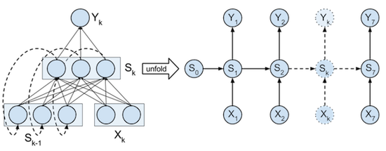
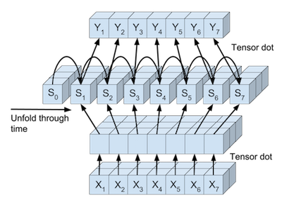
Or we can view the processing of the full input, state-updates, and full output seperately from each other. The full input tensor can be mapped in parallel to be used directly in the RNN state updates. And also the RNN states can be mapped in parallel to the output of each timestep.
The steps are abstracted in different classes below. Each class has a
forward
method that performs the
forward steps
of backpropagation, and a
backward
method that perform the
backward
steps of backpropagation.
Processing of input and output tensors
Linear transformation
Neural networks typically transform input vectors by matrix multiplication and vector addition followed by a non-linear transfer function. The 2-dimensional input vectors to our network $(x_{ik1}$, $x_{ik2})$ are transformed by a $2 \times 3$ weight matrix and a bias vector of size 3. Before they can be added to the states of the RNN. The 3-dimensional state vectors are transformed to a 1-dimensional output vector by a $3 \times 1$ weight matrix and a bias vector of size 1 to give the output probabilities.
Since we want to process all inputs for each sample and each timestep in one computation we can use the numpy
tensordot
function to perform the dot products. This function takes 2 tensors and the axes that need to be aggregated by summation between the elements and a product of the result. For example the transformation of input X ($2000 \times 7 \times 2$) to the states S ($2000 \times 7 \times 3$) with the help of matrix W ($2 \times 3$) can be done by
S = tensordot(X, W, axes=((-1),(0)))
. This method will sum the elements of the last order (-1) of X with the elements of the first order (0) of W and multiply them together. This is the same as doing the matrix dot product for each $[x_{ik1}$, $x_{ik2}]$ vector with W.
tensordot
can then make sure that the underlying computations can be done efficiently and in parallel.
These linear tensor transformations are used to transform the input X to the states S, and from the states S to the output Y. This linear transformation, together with its gradient is implemented in the
TensorLinear
class below. Note that the weights are initialized by sampling uniformly between $\pm \sqrt{6.0 / (n_{in} + n_{out})}$
as suggested by X. Glorot
.
Logistic classification
Logistic classification
is used to output the probability that the output at current time step k is 1. This function together with its loss and gradient is implemented in the
LogisticClassifier
class below.
# Define the linear tensor transformation layer
class TensorLinear(object):
    """The linear tensor layer applies a linear tensor dot product
    and a bias to its input."""
    def __init__(self, n_in, n_out, tensor_order, W=None, b=None):
        """Initialse the weight W and bias b parameters."""
        a = np.sqrt(6.0 / (n_in + n_out))
        self.W = (np.random.uniform(-a, a, (n_in, n_out))
                  if W is None else W)
        self.b = (np.zeros((n_out)) if b is None else b)
        # Axes summed over in backprop
        self.bpAxes = tuple(range(tensor_order-1))

    def forward(self, X):
        """Perform forward step transformation with the help
        of a tensor product."""
        # Same as: Y[i,j,:] = np.dot(X[i,j,:], self.W) + self.b
        #          (for i,j in X.shape[0:1])
        # Same as: Y = np.einsum('ijk,kl->ijl', X, self.W) + self.b
        return np.tensordot(X, self.W, axes=((-1),(0))) + self.b

    def backward(self, X, gY):
        """Return the gradient of the parmeters and the inputs of
        this layer."""
        # Same as: gW = np.einsum('ijk,ijl->kl', X, gY)
        # Same as: gW += np.dot(X[:,j,:].T, gY[:,j,:])
        #          (for i,j in X.shape[0:1])
        gW = np.tensordot(X, gY, axes=(self.bpAxes, self.bpAxes))
        gB = np.sum(gY, axis=self.bpAxes)
        # Same as: gX = np.einsum('ijk,kl->ijl', gY, self.W.T)
        # Same as: gX[i,j,:] = np.dot(gY[i,j,:], self.W.T)
        #          (for i,j in gY.shape[0:1])
        gX = np.tensordot(gY, self.W.T, axes=((-1),(0)))
        return gX, gW, gB
# Define the logistic classifier layer
class LogisticClassifier(object):
    """The logistic layer applies the logistic function to its
    inputs."""

    def forward(self, X):
        """Perform the forward step transformation."""
        return 1. / (1. + np.exp(-X))

    def backward(self, Y, T):
        """Return the gradient with respect to the loss function
        at the inputs of this layer."""
        # Average by the number of samples and sequence length.
        return (Y - T) / (Y.shape[0] * Y.shape[1])

    def loss(self, Y, T):
        """Compute the loss at the output."""
        return -np.mean((T * np.log(Y)) + ((1-T) * np.log(1-Y)))
Unfolding the recurrent states
Just as in the
previous part
of this tutorial the recurrent states need to be unfolded through time. This unfolding during
backpropagation through time
is done by the
RecurrentStateUnfold
class. This class holds the shared weight and bias parameters used to update each state, as well as the initial state that is also treated as a parameter and optimized during backpropagation.
The
forward
method of
RecurrentStateUnfold
iteratively updates the states through time and returns the resulting state tensor. The
backward
method propagates the gradients at the outputs of each state backwards through time. Note that at each time $k$ the gradient coming from the output Y needs to be added with the gradient coming from the previous state at time $k+1$. The gradients of the weight and bias parameters are summed over all timestep since they are shared parameters in each state update. The final state gradient at time $k=0$ is used to optimise the initial state $S_0$ since the gradient of the inital state is $\partial \xi / \partial S_{0}$.
RecurrentStateUnfold
makes use of the
RecurrentStateUpdate
class. The
forward
method of this class combines the transformed input and state at time $k-1$ to output state $k$. The
backward
method propagates the gradient backwards through time for one timestep and calculates the gradients of the parameters of this timestep. The non-linear transfer function used in
RecurrentStateUpdate
is the
hyperbolic tangent
(tanh) function. This function, like the logistic function, is a
sigmoid function
that goes from $-1$ to $+1$. The
tanh function
is chosen because the maximum gradient of this function is higher than the maximum gradient of the
logistic function
which make vanishing gradients less likely. This tanh transfer function is implemented in the
TanH
class.
# Define tanh layer
class TanH(object):
    """TanH applies the tanh function to its inputs."""

    def forward(self, X):
        """Perform the forward step transformation."""
        return np.tanh(X)

    def backward(self, Y, output_grad):
        """Return the gradient at the inputs of this layer."""
        gTanh = 1.0 - (Y**2)
        return (gTanh * output_grad)
# Define internal state update layer
class RecurrentStateUpdate(object):
    """Update a given state."""
    def __init__(self, nbStates, W, b):
        """Initialse the linear transformation and tanh transfer
        function."""
        self.linear = TensorLinear(nbStates, nbStates, 2, W, b)
        self.tanh = TanH()

    def forward(self, Xk, Sk):
        """Return state k+1 from input and state k."""
        return self.tanh.forward(Xk + self.linear.forward(Sk))

    def backward(self, Sk0, Sk1, output_grad):
        """Return the gradient of the parmeters and the inputs of
        this layer."""
        gZ = self.tanh.backward(Sk1, output_grad)
        gSk0, gW, gB = self.linear.backward(Sk0, gZ)
        return gZ, gSk0, gW, gB
# Define layer that unfolds the states over time
class RecurrentStateUnfold(object):
    """Unfold the recurrent states."""
    def __init__(self, nbStates, nbTimesteps):
        """Initialse the shared parameters, the inital state and
        state update function."""
        a = np.sqrt(6. / (nbStates * 2))
        self.W = np.random.uniform(-a, a, (nbStates, nbStates))
        self.b = np.zeros((self.W.shape[0]))  # Shared bias
        self.S0 = np.zeros(nbStates)  # Initial state
        self.nbTimesteps = nbTimesteps  # Timesteps to unfold
        self.stateUpdate = RecurrentStateUpdate(
            nbStates, self.W, self.b)  # State update function

    def forward(self, X):
        """Iteratively apply forward step to all states."""
        # State tensor
        S = np.zeros((X.shape[0], X.shape[1]+1, self.W.shape[0]))
        S[:,0,:] = self.S0  # Set initial state
        for k in range(self.nbTimesteps):
            # Update the states iteratively
            S[:,k+1,:] = self.stateUpdate.forward(X[:,k,:], S[:,k,:])
        return S

    def backward(self, X, S, gY):
        """Return the gradient of the parmeters and the inputs of
        this layer."""
        # Initialise gradient of state outputs
        gSk = np.zeros_like(gY[:,self.nbTimesteps-1,:])
        # Initialse gradient tensor for state inputs
        gZ = np.zeros_like(X)
        gWSum = np.zeros_like(self.W)  # Initialise weight gradients
        gBSum = np.zeros_like(self.b)  # Initialse bias gradients
        # Propagate the gradients iteratively
        for k in range(self.nbTimesteps-1, -1, -1):
            # Gradient at state output is gradient from previous state
            #  plus gradient from output
            gSk += gY[:,k,:]
            # Propgate the gradient back through one state
            gZ[:,k,:], gSk, gW, gB = self.stateUpdate.backward(
                S[:,k,:], S[:,k+1,:], gSk)
            gWSum += gW  # Update total weight gradient
            gBSum += gB  # Update total bias gradient
        # Get gradient of initial state over all samples
        gS0 = np.sum(gSk, axis=0)
        return gZ, gWSum, gBSum, gS0
The full network
The full network that will be trained to perform binary addition of two number is defined in the
RnnBinaryAdder
class below. It initialises all the layers upon creation. The
forward
method performs the full backpropagation forward step through all layers and timesteps and returns the intermediary outputs. The
backward
method performs the backward step through all layers and timesteps and returns the gradients of all the parameters. The
getParamGrads
method performs both steps and returns the gradients of the parameters in a list. The order of this list corresponds to the order of the iterator returned by
get_params_iter
. The parameters returned in the iterator of that last method are the same as the parameters of the network and can be used to change the parameters of the network manually.
# Define the full network
class RnnBinaryAdder(object):
    """RNN to perform binary addition of 2 numbers."""
    def __init__(self, nb_of_inputs, nb_of_outputs, nb_of_states,
                 sequence_len):
        """Initialse the network layers."""
        # Input layer
        self.tensorInput = TensorLinear(nb_of_inputs, nb_of_states, 3)
        # Recurrent layer
        self.rnnUnfold = RecurrentStateUnfold(nb_of_states, sequence_len)
        # Linear output transform
        self.tensorOutput = TensorLinear(nb_of_states, nb_of_outputs, 3)
        self.classifier = LogisticClassifier()  # Classification output

    def forward(self, X):
        """Perform the forward propagation of input X through all
        layers."""
        # Linear input transformation
        recIn = self.tensorInput.forward(X)
        # Forward propagate through time and return states
        S = self.rnnUnfold.forward(recIn)
        # Linear output transformation
        Z = self.tensorOutput.forward(S[:,1:sequence_len+1,:])
        Y = self.classifier.forward(Z)  # Classification probabilities
        # Return: input to recurrent layer, states, input to classifier,
        #  output
        return recIn, S, Z, Y

    def backward(self, X, Y, recIn, S, T):
        """Perform the backward propagation through all layers.
        Input: input samples, network output, intput to recurrent
        layer, states, targets."""
        gZ = self.classifier.backward(Y, T)  # Get output gradient
        gRecOut, gWout, gBout = self.tensorOutput.backward(
            S[:,1:sequence_len+1,:], gZ)
        # Propagate gradient backwards through time
        gRnnIn, gWrec, gBrec, gS0 = self.rnnUnfold.backward(
            recIn, S, gRecOut)
        gX, gWin, gBin = self.tensorInput.backward(X, gRnnIn)
        # Return the parameter gradients of: linear output weights,
        #  linear output bias, recursive weights, recursive bias, #
        #  linear input weights, linear input bias, initial state.
        return gWout, gBout, gWrec, gBrec, gWin, gBin, gS0

    def getOutput(self, X):
        """Get the output probabilities of input X."""
        recIn, S, Z, Y = self.forward(X)
        return Y

    def getBinaryOutput(self, X):
        """Get the binary output of input X."""
        return np.around(self.getOutput(X))

    def getParamGrads(self, X, T):
        """Return the gradients with respect to input X and
        target T as a list. The list has the same order as the
        get_params_iter iterator."""
        recIn, S, Z, Y = self.forward(X)
        gWout, gBout, gWrec, gBrec, gWin, gBin, gS0 = self.backward(
            X, Y, recIn, S, T)
        return [g for g in itertools.chain(
                np.nditer(gS0),
                np.nditer(gWin),
                np.nditer(gBin),
                np.nditer(gWrec),
                np.nditer(gBrec),
                np.nditer(gWout),
                np.nditer(gBout))]

    def loss(self, Y, T):
        """Return the loss of input X w.r.t. targets T."""
        return self.classifier.loss(Y, T)

    def get_params_iter(self):
        """Return an iterator over the parameters.
        The iterator has the same order as get_params_grad.
        The elements returned by the iterator are editable in-place."""
        return itertools.chain(
            np.nditer(self.rnnUnfold.S0, op_flags=['readwrite']),
            np.nditer(self.tensorInput.W, op_flags=['readwrite']),
            np.nditer(self.tensorInput.b, op_flags=['readwrite']),
            np.nditer(self.rnnUnfold.W, op_flags=['readwrite']),
            np.nditer(self.rnnUnfold.b, op_flags=['readwrite']),
            np.nditer(self.tensorOutput.W, op_flags=['readwrite']),
            np.nditer(self.tensorOutput.b, op_flags=['readwrite']))
Gradient Checking
As in part 4 of our previous tutorial on feedforward nets the gradient computed by backpropagation is compared with the numerical gradient to assert that there are no bugs in the code to compute the gradients. This is done by the code below.
# Do gradient checking
# Define an RNN to test
RNN = RnnBinaryAdder(2, 1, 3, sequence_len)
# Get the gradients of the parameters from a subset of the data
backprop_grads = RNN.getParamGrads(
    X_train[0:100,:,:], T_train[0:100,:,:])

eps = 1e-7  # Set the small change to compute the numerical gradient
# Compute the numerical gradients of the parameters in all layers.
for p_idx, param in enumerate(RNN.get_params_iter()):
    grad_backprop = backprop_grads[p_idx]
    # + eps
    param += eps
    plus_loss = RNN.loss(
        RNN.getOutput(X_train[0:100,:,:]), T_train[0:100,:,:])
    # - eps
    param -= 2 * eps
    min_loss = RNN.loss(
        RNN.getOutput(X_train[0:100,:,:]), T_train[0:100,:,:])
    # reset param value
    param += eps
    # calculate numerical gradient
    grad_num = (plus_loss - min_loss) / (2*eps)
    # Raise error if the numerical grade is not close to the
    #  backprop gradient
    if not np.isclose(grad_num, grad_backprop):
        raise ValueError((
            f'Numerical gradient of {grad_num:.6f} is not close '
            f'to the backpropagation gradient of {grad_backprop:.6f}!'
        ))
print('No gradient errors found')
#
Rmsprop with momentum optimisation
While the first part of this tutorial used RProp to optimise the network, this part will use the RMSProp algorithm with Nesterov's accelerated gradient to perform the optimisation. We replaced the Rprop algorithm because Rprop doesn't work well with minibatches due to the stochastic nature of the error surface that can result in sign changes of the gradient.
The Rmsprop algorithm was inspired by the Rprop algorithm. It keeps a
moving average
(MA) of the squared gradient for each parameter $\theta$ ($MA = \lambda \cdot MA + (1-\lambda) \cdot (\partial \xi / \partial \theta)^2$, with $\lambda$ the moving average hyperparameter). The gradient is then normalised by dividing by the square root of this moving average (
maSquare
= $(\partial \xi / \partial \theta)/\sqrt{MA}$). This normalised gradient is then used to update the parameters. Note that if $\lambda=0$ the gradient is reduced to its sign.
This transformed gradient is not used directly to update the parameters, but it is used to update a momentum parameter (
Vs
) for each parameter of the network. This parameter is similar to the momentum parameter from our
previous tutorial
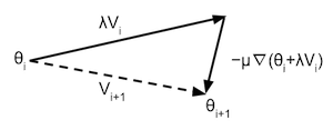
but it is used in a slightly different way. Nesterov's accelerated gradient is different from regular momentum in that it applies updates in a different way. While the regular momentum algorithm calculates the gradient at the beginning of the iteration, updates the momentum and moves the parameters according to this momentum, Nesterov's accelerated gradient moves the parameters according to the reduced momentum, then calculates the gradients, updates the momentum, and then moves again according to the local gradient. This has as benefit that the gradient is more informative to do the local update, and can correct for a bad momentum update. The Nesterov updates can be described as:
With $\nabla(\theta)$ the local gradient at position $\theta$ in the parameter space. And $i$ the iteration number. This formula can be visualised as in the following illustration (See Sutskever I. ):
Note that the training converges to a loss of 0. This convergence is actually not guaranteed. If the parameters of the network start out in a bad position the network might convert to a local minimum that is far from the global minimum. The training is also sensitive to the meta parameters
lmbd
,
learning_rate
,
momentum_term
,
eps
. Try rerunning this yourself to see how many times it actually converges.
# Set hyper-parameters
lmbd = 0.5  # Rmsprop lambda
learning_rate = 0.05  # Learning rate
momentum_term = 0.80  # Momentum term
eps = 1e-6  # Numerical stability term to prevent division by zero
mb_size = 100  # Size of the minibatches (number of samples)

# Create the network
nb_of_states = 3  # Number of states in the recurrent layer
RNN = RnnBinaryAdder(2, 1, nb_of_states, sequence_len)
# Set the initial parameters
# Number of parameters in the network
nbParameters =  sum(1 for _ in RNN.get_params_iter())
# Rmsprop moving average
maSquare = [0.0 for _ in range(nbParameters)]
Vs = [0.0 for _ in range(nbParameters)]  # Momentum

# Create a list of minibatch losses to be plotted
ls_of_loss = [
    RNN.loss(RNN.getOutput(X_train[0:100,:,:]), T_train[0:100,:,:])]
# Iterate over some iterations
for i in range(5):
    # Iterate over all the minibatches
    for mb in range(nb_train // mb_size):
        X_mb = X_train[mb:mb+mb_size,:,:]  # Input minibatch
        T_mb = T_train[mb:mb+mb_size,:,:]  # Target minibatch
        V_tmp = [v * momentum_term for v in Vs]
        # Update each parameters according to previous gradient
        for pIdx, P in enumerate(RNN.get_params_iter()):
            P += V_tmp[pIdx]
        # Get gradients after following old velocity
        # Get the parameter gradients
        backprop_grads = RNN.getParamGrads(X_mb, T_mb)
        # Update each parameter seperately
        for pIdx, P in enumerate(RNN.get_params_iter()):
            # Update the Rmsprop moving averages
            maSquare[pIdx] = lmbd * maSquare[pIdx] + (
                1-lmbd) * backprop_grads[pIdx]**2
            # Calculate the Rmsprop normalised gradient
            pGradNorm = ((
                learning_rate * backprop_grads[pIdx]) / np.sqrt(
                maSquare[pIdx]) + eps)
            # Update the momentum
            Vs[pIdx] = V_tmp[pIdx] - pGradNorm
            P -= pGradNorm   # Update the parameter
        # Add loss to list to plot
        ls_of_loss.append(RNN.loss(RNN.getOutput(X_mb), T_mb))
# Plot the loss over the iterations
fig = plt.figure(figsize=(5, 3))
plt.plot(ls_of_loss, 'b-')
plt.xlabel('minibatch iteration')
plt.ylabel('$\\xi$', fontsize=15)
plt.title('Decrease of loss over backprop iteration')
plt.xlim(0, 100)
fig.subplots_adjust(bottom=0.2)
plt.show()
#
Test examples
The figure above shows that the training converged to a loss of 0. We expect the network to have learned how to perfectly do binary addition for our training examples. If we put some independent test cases through the network and print them out we can see that the network also outputs the correct output for these test cases.
# Create test samples
nb_test = 5
Xtest, Ttest = create_dataset(nb_test, sequence_len)
# Push test data through network
Y = RNN.getBinaryOutput(Xtest)
Yf = RNN.getOutput(Xtest)

# Print out all test examples
for i in range(Xtest.shape[0]):
    printSample(Xtest[i,:,0], Xtest[i,:,1], Ttest[i,:,:], Y[i,:,:])
    print('')
#
This was the last part of a 2-part tutorial on how to implement an RNN from scratch in Python and NumPy:
# Python package versions used
%load_ext watermark
%watermark --python
%watermark --iversions
#
This post at peterroelants.github.io is generated from an IPython notebook file. Link to the full IPython notebook file
Neural Networks Recurrent Neural Network (RNN) Machine Learning NumPy RMSProp Nonlinearity Nesterov momentum Sequential Data Notebook